Motion Control
The robot’s movement system is based on a three-motor omnidirectional base, allowing it to move in any direction without needing to rotate first. This flexibility is crucial for quick responses and smooth navigation in dynamic environments, such as robotic competitions.
Velocity Equations for an Omnidirectional Base
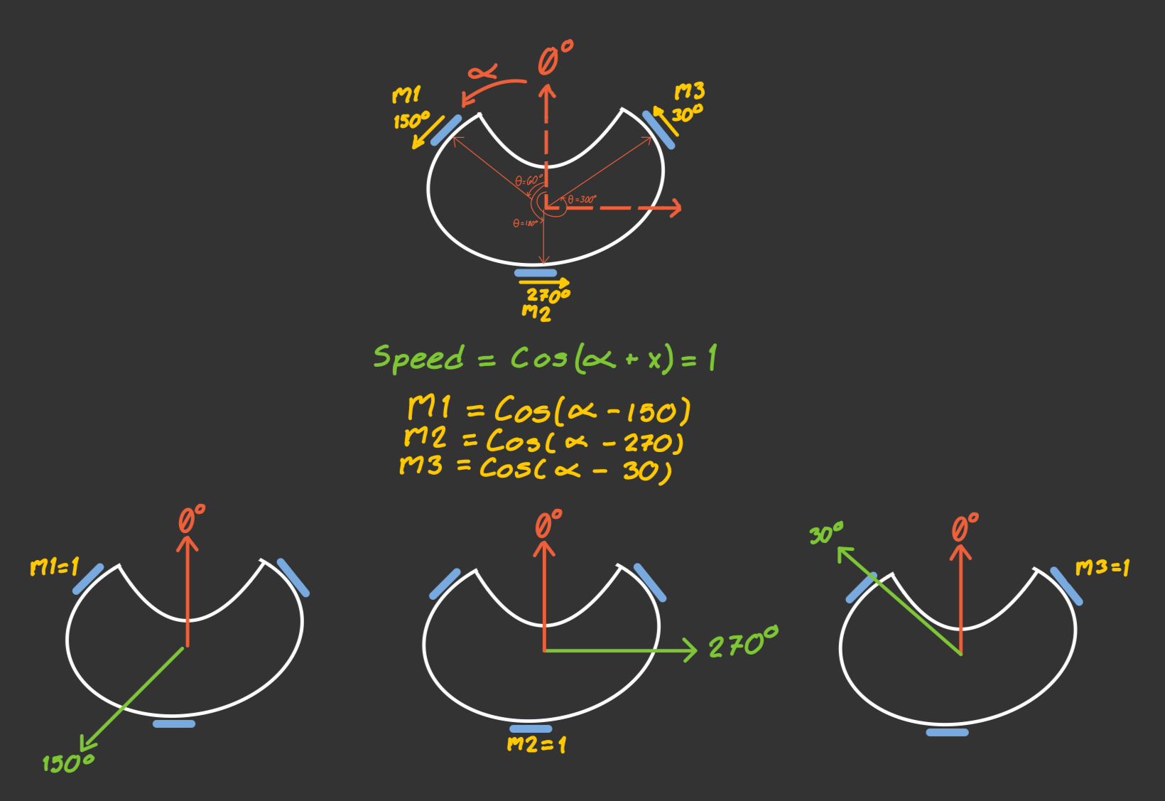
The equations that describe the movement of an omnidirectional base rely themselves on trigonometry and the specific configuration of the motors. Each motor contributes to the overall movement of the robot in a way that can be mathematically modeled using cosine functions.
Each and every single motor have a \(\Delta\phi\) of \(120^{\circ}\); located each at \(60^{\circ}\), \(180^{\circ}\), and \(300^{\circ}\) respectively from where the robot is facing forward. Since the wheels are mounted perpendicular to the axis of each motor, we need to add \(90^{\circ}\) to each of these angles to get the direction in which each motor contributes to the movement of the robot. Granting us the following angles for each motor:
- Motor m1: \(150^{\circ}\)
- Motor m2: \(270^{\circ}\)
- Motor m3: \(30^{\circ}\)
Before we explain how we calculate the speed at which a motor moves, it is important to introduce the concept of torque and how it relates to the velocity of the robot. We are able to communicate to the drivers to set a certain speed by using PWM. However, this is not what's actually occuring on the physical level. The motors have a certain torque curve, which means that they will only start moving at a certain minimum PWM value. If we neglect this fact, it can lead to scenarios where we command the robot to move, but since it's unable to move at that PWM value, it will remain at rest.
With that in mind, in order to calculate the speed of each motor, we need to take into account the direction at which we want the robot to move. We can represent this with the following general expression:
Where:
- \(\theta\) is the direction we want the robot to move (parameter we'll introduce),
- \(\phi_i\) is the direction in which each motor contributes movement (Value we need to find),
- \(v\) is the normalized speed of motor, with values between
-1and1.
In the end, we end up with the following model for the speed of each motor based on the desired movement direction \(\theta\):
\(P_1 = v\cos(\theta - 150^{\circ})\)
\(P_2 = v\cos(\theta - 270^{\circ})\)
\(P_3 = v\cos(\theta - 30^{\circ})\)
These equations are now able to give us the speed of each motor based on where we want the robot to move. For example, if we want the robot to move forward, we would set \(\theta\) to \(0^{\circ}\). If we want the robot to move to the right, we would set \(\theta\) to \(90^{\circ}\). By adjusting \(\theta\), we can command the robot to move in any direction.
In code, to compute each motor’s speed, we use the following method:
void Motors::move(float angleDegrees, float speedPercent, float rotationalSpeed) {
    float upper_left_speed = cos((angleDegrees - 150) * PI / 180.0f) * speedPercent + rotationalSpeed;
    float lower_center_speed = cos((angleDegrees - 270) * PI / 180.0f) * speedPercent + rotationalSpeed;
    float upper_right_speed = cos((angleDegrees - 30) * PI / 180.0f) * speedPercent + rotationalSpeed;

    left.setSpeed(upper_left_speed);
    center.setSpeed(lower_center_speed);
    right.setSpeed(upper_right_speed);
}
SetSpeed() is the method that takes care of each individual motor object; moving the motor to a desired speed and the direction (forward or backwards) to a desired speed.
void Motor::setSpeed(float speed) {
    if (speed > 0.0f) {
        speed += GetMotorSpeedOffset(id);
    } else if (speed < 0.0f) {
        speed -= GetMotorSpeedOffset(id);
    }

    speed = constrain(speed, -255.0f, 255.0f);

    if (abs(speed) < 1.0f) {
        analogWrite(pwmPin, 0);
        return;
    }

    if (speed < 0) {
        digitalWrite(in1Pin, LOW);
        digitalWrite(in2Pin, HIGH);
    } else {
        digitalWrite(in1Pin, HIGH);
        digitalWrite(in2Pin, LOW);
    }

    analogWrite(pwmPin, (int)abs(speed));
}
PID Controller
As a fundamental part of the robot structure, in order for the robot to be able to score, it needs to be pointing to the right direction. In order to control to where the robot is facing, you need to use the aformentioned move method with it's respective rotationalSpeed. This, traditionally has always been done by using a PID.
The formula to calculate the PID for any given function is a classical result from control theory; showing up on this classical form:
The issue with using this classical result is the fact that sometimes you can land on valleys. If you got a PID that's calibrated high on \(P\), on small differences between origin angle and current angle \((\Delta \theta)\), you will overshoot. If we add an \(I\) parameter, this should do the trick. However, motors don't move at any PWM values, they need to move at minimum speed, otherwise the robot will literally not move. The result now is that you will not overshoot if you are over a certain large \(\Delta \theta\), but you will not arrive if \(\Delta \theta\) is small enough. You can try to combat this by increasing \(I\), however, now you have the same problem but in reverse. At large \(\Delta \theta\) you will overshoot, while at small \(\Delta \theta\) you will reach a certain value. It's is plausible to believe that it's just matter of proper calibration, however, there's a linear asymptote that prevents this from happening in the traditional model. Even if it was possible, it would be so sensible to initial conditions, that the second it exited the routine (i.e: when the robot detects line), the \(I\) parameter will make the robot move uncontrollably.
In order to fight this problem, a solution is to add a step function that will only activate if and only if \(\Delta \theta\) is inside within a certain domain.
Such mathematical model can be define in the following fashion by using this piecewise model:
The result of using this approach, is that now we are able to use more agressive models, since the deadbands protect us from accidentally losing control. Using this approach, we are able to calibrate our model, as we only really need to calibrate two values \(K_p\) and \(K_d\), deadbands and limits can be set based on the physical properties of the robot, and the \(I\) parameter can be set to zero, since we don't have to worry about landing on valleys.